


Almost Sure
@almostsure.bsky.social
George Lowther. Author of Almost Sure blog on maths, probability and stochastic calculus
https://almostsuremath.com
Also on YouTube: https://www.youtube.com/@almostsure
https://almostsuremath.com
Also on YouTube: https://www.youtube.com/@almostsure

Inaugural Board of Peace meeting is under way
January 22, 2026 at 10:58 AM
Inaugural Board of Peace meeting is under way
Hey US-Americans, can you just give Trump Alaska? He won’t know the difference and might keep him quiet for a bit
January 21, 2026 at 4:01 PM
Hey US-Americans, can you just give Trump Alaska? He won’t know the difference and might keep him quiet for a bit
“do you even lift bro?”

January 18, 2026 at 8:56 PM
“do you even lift bro?”
January 18, 2026 at 3:15 PM
Woke up to this sight

January 16, 2026 at 8:26 PM
Woke up to this sight
hey everyone!
I won the knowbell prize!
I won the knowbell prize!
January 16, 2026 at 4:14 PM
hey everyone!
I won the knowbell prize!
I won the knowbell prize!
Kids are really cute when they’re at that age where they haven’t yet worked out that giving you their snack means less for them
January 16, 2026 at 3:49 PM
Kids are really cute when they’re at that age where they haven’t yet worked out that giving you their snack means less for them
hey @johnbull.wtf you can’t just post this and delete it!

January 14, 2026 at 4:34 PM
hey @johnbull.wtf you can’t just post this and delete it!
A second hand yacht? Really? How poor do they think we are?

January 14, 2026 at 4:30 PM
A second hand yacht? Really? How poor do they think we are?
so how hard are these Erdös problems anyway?
January 14, 2026 at 4:24 PM
so how hard are these Erdös problems anyway?
Land line
analogue tape
analogue clock
real life
analogue tape
analogue clock
real life

Acoustic guitars used to just be called ‘guitars.’
Then, we invented electric guitars. Oh no.
Which meant saying ‘guitar’ wasn’t clear enough.
So 'guitars' became 'acoustic guitars.'
‘Acoustic guitar’ is an example of a ‘retronym.’
🧵⬇️
Then, we invented electric guitars. Oh no.
Which meant saying ‘guitar’ wasn’t clear enough.
So 'guitars' became 'acoustic guitars.'
‘Acoustic guitar’ is an example of a ‘retronym.’
🧵⬇️
January 13, 2026 at 11:40 PM
Land line
analogue tape
analogue clock
real life
analogue tape
analogue clock
real life
You’re probably familiar with Fourier transforms. But, did you know that it can be viewed as a 90° rotation in the time-frequency domain and we can rotate by any angle via fractional Fourier transform.
Explains why applying FT twice gives reflection (rotation by 180°).
Explains why applying FT twice gives reflection (rotation by 180°).

January 12, 2026 at 1:57 PM
You’re probably familiar with Fourier transforms. But, did you know that it can be viewed as a 90° rotation in the time-frequency domain and we can rotate by any angle via fractional Fourier transform.
Explains why applying FT twice gives reflection (rotation by 180°).
Explains why applying FT twice gives reflection (rotation by 180°).
Ghost fox?
So the other night a fox came up to me with a tennis ball in its mouth. Quite unusual so tried taking a picture, but fumbled trying to select camera app and it was already walking away by the time I was ready.
But why can you see through it?
So the other night a fox came up to me with a tennis ball in its mouth. Quite unusual so tried taking a picture, but fumbled trying to select camera app and it was already walking away by the time I was ready.
But why can you see through it?

January 12, 2026 at 1:44 PM
Ghost fox?
So the other night a fox came up to me with a tennis ball in its mouth. Quite unusual so tried taking a picture, but fumbled trying to select camera app and it was already walking away by the time I was ready.
But why can you see through it?
So the other night a fox came up to me with a tennis ball in its mouth. Quite unusual so tried taking a picture, but fumbled trying to select camera app and it was already walking away by the time I was ready.
But why can you see through it?
“jones dual” to avoid confusion

Just heard a sports reporter on the radio pronounce "cojones" as "ker-Jones" and now I need to burn the radio.
January 12, 2026 at 10:01 AM
“jones dual” to avoid confusion
Anyone had success using AI to help generate Manim animations?
I tried Claude, but due to autocorrect (Manim->mania…) it used JavaScript, and produced nice results.
But when I asked to do in Manim, was full of bugs, did not do the correct thing when these were fixed, and eventually it gave up
I tried Claude, but due to autocorrect (Manim->mania…) it used JavaScript, and produced nice results.
But when I asked to do in Manim, was full of bugs, did not do the correct thing when these were fixed, and eventually it gave up
January 9, 2026 at 5:27 PM
Anyone had success using AI to help generate Manim animations?
I tried Claude, but due to autocorrect (Manim->mania…) it used JavaScript, and produced nice results.
But when I asked to do in Manim, was full of bugs, did not do the correct thing when these were fixed, and eventually it gave up
I tried Claude, but due to autocorrect (Manim->mania…) it used JavaScript, and produced nice results.
But when I asked to do in Manim, was full of bugs, did not do the correct thing when these were fixed, and eventually it gave up
cool 2026 fact: it’s a sum of just two primes!
January 2, 2026 at 8:38 PM
cool 2026 fact: it’s a sum of just two primes!
New YouTube video uploaded on connections between Riemann zeta and Brownian motion!
What does Riemann Zeta have to do with Brownian Motion?
youtu.be/YTQKbgxbtiw
What does Riemann Zeta have to do with Brownian Motion?
youtu.be/YTQKbgxbtiw

What does Riemann Zeta have to do with Brownian Motion?
YouTube video by Almost Sure
youtu.be
November 9, 2025 at 8:19 PM
New YouTube video uploaded on connections between Riemann zeta and Brownian motion!
What does Riemann Zeta have to do with Brownian Motion?
youtu.be/YTQKbgxbtiw
What does Riemann Zeta have to do with Brownian Motion?
youtu.be/YTQKbgxbtiw
It's a while since my last YT video upload. Nothing is happening, I am busy working on the next one. Just taking longer than expected (been very busy recent weekends).
Will be on connections between Riemann zeta and Brownian motion.
ETA a few days to a week.
Will be on connections between Riemann zeta and Brownian motion.
ETA a few days to a week.

November 2, 2025 at 1:15 PM
It's a while since my last YT video upload. Nothing is happening, I am busy working on the next one. Just taking longer than expected (been very busy recent weekends).
Will be on connections between Riemann zeta and Brownian motion.
ETA a few days to a week.
Will be on connections between Riemann zeta and Brownian motion.
ETA a few days to a week.
New YouTube video: Wild Expectations!
This looks at weird properties of conditional expectations, such as two random variables being bigger than each other 'on average'
youtu.be/4ZwRXVVepj8?...
This looks at weird properties of conditional expectations, such as two random variables being bigger than each other 'on average'
youtu.be/4ZwRXVVepj8?...

Wild Expectations
YouTube video by Almost Sure
youtu.be
September 23, 2025 at 8:59 PM
New YouTube video: Wild Expectations!
This looks at weird properties of conditional expectations, such as two random variables being bigger than each other 'on average'
youtu.be/4ZwRXVVepj8?...
This looks at weird properties of conditional expectations, such as two random variables being bigger than each other 'on average'
youtu.be/4ZwRXVVepj8?...
Whatever you do, 𝙛𝙤𝙧 𝙩𝙝𝙚 𝙡𝙤𝙫𝙚 𝙤𝙛 𝙂𝙤𝙙, do not ask random variables to be Lebesgue measurable!
If you were so stupid to do that, then 𝙮𝙤𝙪 𝙬𝙤𝙪𝙡𝙙 𝙣𝙤𝙩 𝙚𝙫𝙚𝙣 𝙗𝙚 𝙖𝙗𝙡𝙚 𝙩𝙤 𝙖𝙙𝙙 𝙧𝙖𝙣𝙙𝙤𝙢 𝙫𝙖𝙧𝙞𝙖𝙗𝙡𝙚𝙨 𝙩𝙤𝙜𝙚𝙩𝙝𝙚𝙧.
If you were so stupid to do that, then 𝙮𝙤𝙪 𝙬𝙤𝙪𝙡𝙙 𝙣𝙤𝙩 𝙚𝙫𝙚𝙣 𝙗𝙚 𝙖𝙗𝙡𝙚 𝙩𝙤 𝙖𝙙𝙙 𝙧𝙖𝙣𝙙𝙤𝙢 𝙫𝙖𝙧𝙞𝙖𝙗𝙡𝙚𝙨 𝙩𝙤𝙜𝙚𝙩𝙝𝙚𝙧.


September 18, 2025 at 8:36 PM
Whatever you do, 𝙛𝙤𝙧 𝙩𝙝𝙚 𝙡𝙤𝙫𝙚 𝙤𝙛 𝙂𝙤𝙙, do not ask random variables to be Lebesgue measurable!
If you were so stupid to do that, then 𝙮𝙤𝙪 𝙬𝙤𝙪𝙡𝙙 𝙣𝙤𝙩 𝙚𝙫𝙚𝙣 𝙗𝙚 𝙖𝙗𝙡𝙚 𝙩𝙤 𝙖𝙙𝙙 𝙧𝙖𝙣𝙙𝙤𝙢 𝙫𝙖𝙧𝙞𝙖𝙗𝙡𝙚𝙨 𝙩𝙤𝙜𝙚𝙩𝙝𝙚𝙧.
If you were so stupid to do that, then 𝙮𝙤𝙪 𝙬𝙤𝙪𝙡𝙙 𝙣𝙤𝙩 𝙚𝙫𝙚𝙣 𝙗𝙚 𝙖𝙗𝙡𝙚 𝙩𝙤 𝙖𝙙𝙙 𝙧𝙖𝙣𝙙𝙤𝙢 𝙫𝙖𝙧𝙞𝙖𝙗𝙡𝙚𝙨 𝙩𝙤𝙜𝙚𝙩𝙝𝙚𝙧.
New video released on mixing quantum and classical probabilities.
The Algebra of Mixed Quantum States
youtu.be/K6h62Gr0nwg
The Algebra of Mixed Quantum States
youtu.be/K6h62Gr0nwg
The Algebra of Mixed Quantum States
YouTube video by Almost Sure
youtu.be
August 23, 2025 at 3:56 PM
New video released on mixing quantum and classical probabilities.
The Algebra of Mixed Quantum States
youtu.be/K6h62Gr0nwg
The Algebra of Mixed Quantum States
youtu.be/K6h62Gr0nwg
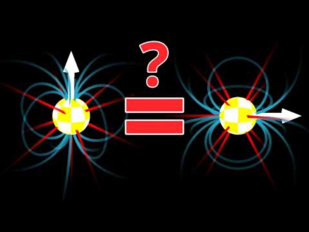
New video released on the Gaussian correlation inequality.
This unexpected proof shocked mathematicians!
youtu.be/WJGR1oc6Gxo?...
This unexpected proof shocked mathematicians!
youtu.be/WJGR1oc6Gxo?...

This unexpected proof shocked mathematicians
YouTube video by Almost Sure
youtu.be
July 3, 2025 at 12:47 PM
New video released on the Gaussian correlation inequality.
This unexpected proof shocked mathematicians!
youtu.be/WJGR1oc6Gxo?...
This unexpected proof shocked mathematicians!
youtu.be/WJGR1oc6Gxo?...
I am not sure if the distribution is symmetric under
X(mu,t)->1-X(1-mu,t).
It is for individual times, as it matches Dirichlet distribution, but probably not for the entire paths wrt t. Which is disappointing. Maybe it can be modified?
X(mu,t)->1-X(1-mu,t).
It is for individual times, as it matches Dirichlet distribution, but probably not for the entire paths wrt t. Which is disappointing. Maybe it can be modified?
Simulating the martingales X(μ,t) which are beta distributed and martingale wrt t.
X(μ,t) ~ Beta(μ(1-t)/t, (1-μ)(1-t)/t)
The (1-t)/t scaling is so that on range 0<t<1 we cover entire set of Beta distributions.
For each t, X(μ_{i+1},t)-X(μ_i,t) have Dirichlet distribution.
X(μ,t) ~ Beta(μ(1-t)/t, (1-μ)(1-t)/t)
The (1-t)/t scaling is so that on range 0<t<1 we cover entire set of Beta distributions.
For each t, X(μ_{i+1},t)-X(μ_i,t) have Dirichlet distribution.
April 17, 2025 at 9:14 AM
I am not sure if the distribution is symmetric under
X(mu,t)->1-X(1-mu,t).
It is for individual times, as it matches Dirichlet distribution, but probably not for the entire paths wrt t. Which is disappointing. Maybe it can be modified?
X(mu,t)->1-X(1-mu,t).
It is for individual times, as it matches Dirichlet distribution, but probably not for the entire paths wrt t. Which is disappointing. Maybe it can be modified?