


Almost Sure
@almostsure.bsky.social
George Lowther. Author of Almost Sure blog on maths, probability and stochastic calculus
https://almostsuremath.com
Also on YouTube: https://www.youtube.com/@almostsure
https://almostsuremath.com
Also on YouTube: https://www.youtube.com/@almostsure
It's a while since my last YT video upload. Nothing is happening, I am busy working on the next one. Just taking longer than expected (been very busy recent weekends).
Will be on connections between Riemann zeta and Brownian motion.
ETA a few days to a week.
Will be on connections between Riemann zeta and Brownian motion.
ETA a few days to a week.

November 2, 2025 at 1:15 PM
It's a while since my last YT video upload. Nothing is happening, I am busy working on the next one. Just taking longer than expected (been very busy recent weekends).
Will be on connections between Riemann zeta and Brownian motion.
ETA a few days to a week.
Will be on connections between Riemann zeta and Brownian motion.
ETA a few days to a week.
I posted this as a YouTube short, so I’ll refer to my description there

October 5, 2025 at 10:31 PM
I posted this as a YouTube short, so I’ll refer to my description there
Whatever you do, 𝙛𝙤𝙧 𝙩𝙝𝙚 𝙡𝙤𝙫𝙚 𝙤𝙛 𝙂𝙤𝙙, do not ask random variables to be Lebesgue measurable!
If you were so stupid to do that, then 𝙮𝙤𝙪 𝙬𝙤𝙪𝙡𝙙 𝙣𝙤𝙩 𝙚𝙫𝙚𝙣 𝙗𝙚 𝙖𝙗𝙡𝙚 𝙩𝙤 𝙖𝙙𝙙 𝙧𝙖𝙣𝙙𝙤𝙢 𝙫𝙖𝙧𝙞𝙖𝙗𝙡𝙚𝙨 𝙩𝙤𝙜𝙚𝙩𝙝𝙚𝙧.
If you were so stupid to do that, then 𝙮𝙤𝙪 𝙬𝙤𝙪𝙡𝙙 𝙣𝙤𝙩 𝙚𝙫𝙚𝙣 𝙗𝙚 𝙖𝙗𝙡𝙚 𝙩𝙤 𝙖𝙙𝙙 𝙧𝙖𝙣𝙙𝙤𝙢 𝙫𝙖𝙧𝙞𝙖𝙗𝙡𝙚𝙨 𝙩𝙤𝙜𝙚𝙩𝙝𝙚𝙧.


September 18, 2025 at 8:36 PM
Whatever you do, 𝙛𝙤𝙧 𝙩𝙝𝙚 𝙡𝙤𝙫𝙚 𝙤𝙛 𝙂𝙤𝙙, do not ask random variables to be Lebesgue measurable!
If you were so stupid to do that, then 𝙮𝙤𝙪 𝙬𝙤𝙪𝙡𝙙 𝙣𝙤𝙩 𝙚𝙫𝙚𝙣 𝙗𝙚 𝙖𝙗𝙡𝙚 𝙩𝙤 𝙖𝙙𝙙 𝙧𝙖𝙣𝙙𝙤𝙢 𝙫𝙖𝙧𝙞𝙖𝙗𝙡𝙚𝙨 𝙩𝙤𝙜𝙚𝙩𝙝𝙚𝙧.
If you were so stupid to do that, then 𝙮𝙤𝙪 𝙬𝙤𝙪𝙡𝙙 𝙣𝙤𝙩 𝙚𝙫𝙚𝙣 𝙗𝙚 𝙖𝙗𝙡𝙚 𝙩𝙤 𝙖𝙙𝙙 𝙧𝙖𝙣𝙙𝙤𝙢 𝙫𝙖𝙧𝙞𝙖𝙗𝙡𝙚𝙨 𝙩𝙤𝙜𝙚𝙩𝙝𝙚𝙧.
Here's the method of simulation, and also shows that the joint distribution of X(μ,t) is uniquely determined if we impose independent ratios property wrt μ.


April 16, 2025 at 2:02 AM
Here's the method of simulation, and also shows that the joint distribution of X(μ,t) is uniquely determined if we impose independent ratios property wrt μ.
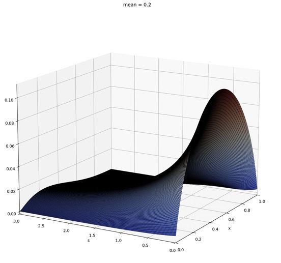
here's another plot (more 'mu' points, fewer time points.
And, gamma(1) process scaled to hit 1 at time 1 (time parameter mu to compare). Corresponds to t=0.5 in the surface plot. You can see its dominated by a few large jumps.
gamma(40) process is shown in the 3rd plot, corresponds with t=0.024
And, gamma(1) process scaled to hit 1 at time 1 (time parameter mu to compare). Corresponds to t=0.5 in the surface plot. You can see its dominated by a few large jumps.
gamma(40) process is shown in the 3rd plot, corresponds with t=0.024


April 15, 2025 at 7:48 PM
here's another plot (more 'mu' points, fewer time points.
And, gamma(1) process scaled to hit 1 at time 1 (time parameter mu to compare). Corresponds to t=0.5 in the surface plot. You can see its dominated by a few large jumps.
gamma(40) process is shown in the 3rd plot, corresponds with t=0.024
And, gamma(1) process scaled to hit 1 at time 1 (time parameter mu to compare). Corresponds to t=0.5 in the surface plot. You can see its dominated by a few large jumps.
gamma(40) process is shown in the 3rd plot, corresponds with t=0.024
Simulating the martingales X(μ,t) which are beta distributed and martingale wrt t.
X(μ,t) ~ Beta(μ(1-t)/t, (1-μ)(1-t)/t)
The (1-t)/t scaling is so that on range 0<t<1 we cover entire set of Beta distributions.
For each t, X(μ_{i+1},t)-X(μ_i,t) have Dirichlet distribution.
X(μ,t) ~ Beta(μ(1-t)/t, (1-μ)(1-t)/t)
The (1-t)/t scaling is so that on range 0<t<1 we cover entire set of Beta distributions.
For each t, X(μ_{i+1},t)-X(μ_i,t) have Dirichlet distribution.


April 15, 2025 at 7:20 PM
Simulating the martingales X(μ,t) which are beta distributed and martingale wrt t.
X(μ,t) ~ Beta(μ(1-t)/t, (1-μ)(1-t)/t)
The (1-t)/t scaling is so that on range 0<t<1 we cover entire set of Beta distributions.
For each t, X(μ_{i+1},t)-X(μ_i,t) have Dirichlet distribution.
X(μ,t) ~ Beta(μ(1-t)/t, (1-μ)(1-t)/t)
The (1-t)/t scaling is so that on range 0<t<1 we cover entire set of Beta distributions.
For each t, X(μ_{i+1},t)-X(μ_i,t) have Dirichlet distribution.
Probability fact:
If X,Y are independent Gamma(a), Gamma(b) random variables then
X/(X+Y), X+Y
are independent Beta(a,b), Gamma(a+b) rvs.
Equivalently: if X,Y are independent Beta(a,b), Gamma(a+b) random variables then
XY, (1-X)Y
are independent Gamma(a), Gamma(b) rvs.
If X,Y are independent Gamma(a), Gamma(b) random variables then
X/(X+Y), X+Y
are independent Beta(a,b), Gamma(a+b) rvs.
Equivalently: if X,Y are independent Beta(a,b), Gamma(a+b) random variables then
XY, (1-X)Y
are independent Gamma(a), Gamma(b) rvs.

April 12, 2025 at 5:33 PM
Probability fact:
If X,Y are independent Gamma(a), Gamma(b) random variables then
X/(X+Y), X+Y
are independent Beta(a,b), Gamma(a+b) rvs.
Equivalently: if X,Y are independent Beta(a,b), Gamma(a+b) random variables then
XY, (1-X)Y
are independent Gamma(a), Gamma(b) rvs.
If X,Y are independent Gamma(a), Gamma(b) random variables then
X/(X+Y), X+Y
are independent Beta(a,b), Gamma(a+b) rvs.
Equivalently: if X,Y are independent Beta(a,b), Gamma(a+b) random variables then
XY, (1-X)Y
are independent Gamma(a), Gamma(b) rvs.
My extension of Hermite-Hadamard:
If c = (pa+qb)/(p+q) for p,q > 0 then
f(c)≤M(t)≤(pf(a)+qf(b))/(p+q)
where M(t) is the average value of f under Beta(qt,pt) distribution scaled to interval [a,b].
M(t) is ctsly decreasing from
M(0)=(pf(a)+qf(b))/(p+q)
to
M(∞) = f(c)
pbs.twimg.com/media/GoSUpd...
If c = (pa+qb)/(p+q) for p,q > 0 then
f(c)≤M(t)≤(pf(a)+qf(b))/(p+q)
where M(t) is the average value of f under Beta(qt,pt) distribution scaled to interval [a,b].
M(t) is ctsly decreasing from
M(0)=(pf(a)+qf(b))/(p+q)
to
M(∞) = f(c)
pbs.twimg.com/media/GoSUpd...

April 12, 2025 at 4:50 PM
My extension of Hermite-Hadamard:
If c = (pa+qb)/(p+q) for p,q > 0 then
f(c)≤M(t)≤(pf(a)+qf(b))/(p+q)
where M(t) is the average value of f under Beta(qt,pt) distribution scaled to interval [a,b].
M(t) is ctsly decreasing from
M(0)=(pf(a)+qf(b))/(p+q)
to
M(∞) = f(c)
pbs.twimg.com/media/GoSUpd...
If c = (pa+qb)/(p+q) for p,q > 0 then
f(c)≤M(t)≤(pf(a)+qf(b))/(p+q)
where M(t) is the average value of f under Beta(qt,pt) distribution scaled to interval [a,b].
M(t) is ctsly decreasing from
M(0)=(pf(a)+qf(b))/(p+q)
to
M(∞) = f(c)
pbs.twimg.com/media/GoSUpd...
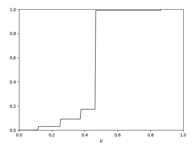
Question: fixed a, b > 0, are distributions Beta(at,bt) decreasing in convex order over t > 0?
Equivalent to existence of a reverse-time martingale X_t ~ Beta(at,bt).
Equivalently:
-(d/dt)E[(x-X_t)_+] >=0
for all 0 < x < 1.
Plots suggest so: parameterised as s=a+b,mean=a/s
Equivalent to existence of a reverse-time martingale X_t ~ Beta(at,bt).
Equivalently:
-(d/dt)E[(x-X_t)_+] >=0
for all 0 < x < 1.
Plots suggest so: parameterised as s=a+b,mean=a/s


April 12, 2025 at 2:49 PM
Question: fixed a, b > 0, are distributions Beta(at,bt) decreasing in convex order over t > 0?
Equivalent to existence of a reverse-time martingale X_t ~ Beta(at,bt).
Equivalently:
-(d/dt)E[(x-X_t)_+] >=0
for all 0 < x < 1.
Plots suggest so: parameterised as s=a+b,mean=a/s
Equivalent to existence of a reverse-time martingale X_t ~ Beta(at,bt).
Equivalently:
-(d/dt)E[(x-X_t)_+] >=0
for all 0 < x < 1.
Plots suggest so: parameterised as s=a+b,mean=a/s
“Reciprocal tariffs”

April 4, 2025 at 9:18 AM
“Reciprocal tariffs”
This later quote does sound negative, although in context it’s not so bad. You wouldn’t start students off on the most general class of cts functions, that are nowhere differentiable, without first mastering smooth functions, would lose sight of why cts functions were introduced in the first place

March 21, 2025 at 5:15 PM
This later quote does sound negative, although in context it’s not so bad. You wouldn’t start students off on the most general class of cts functions, that are nowhere differentiable, without first mastering smooth functions, would lose sight of why cts functions were introduced in the first place
Maybe you’ve heard that Henri Poincaré said that Weierstrass' work (on continuous functions without derivatives) is "an outrage against common sense".
That’s what Wikipedia, and many other sources say. But, no!
Looking up the original source, he's actually being positive about Weierstrass' work!
That’s what Wikipedia, and many other sources say. But, no!
Looking up the original source, he's actually being positive about Weierstrass' work!


March 21, 2025 at 4:57 PM
Maybe you’ve heard that Henri Poincaré said that Weierstrass' work (on continuous functions without derivatives) is "an outrage against common sense".
That’s what Wikipedia, and many other sources say. But, no!
Looking up the original source, he's actually being positive about Weierstrass' work!
That’s what Wikipedia, and many other sources say. But, no!
Looking up the original source, he's actually being positive about Weierstrass' work!
It is Hölder continuous with exponent 1/2. Unlike Brownian motion, which is only locally Hölder continuous for exponents 1/2-ε

March 21, 2025 at 1:34 AM
It is Hölder continuous with exponent 1/2. Unlike Brownian motion, which is only locally Hölder continuous for exponents 1/2-ε
Fractional Brownian motion, varying the Hurst parameter H between 0 and 1. H=0.5 corresponds with standard Brownian motion, and the path has fractal dimension 2-H
March 21, 2025 at 1:22 AM
Fractional Brownian motion, varying the Hurst parameter H between 0 and 1. H=0.5 corresponds with standard Brownian motion, and the path has fractal dimension 2-H
Constructing Weierstrass' function.
Continuous, nowhere differentiable, unbounded variation, no intervals of increase or decrease. Fractal dimension 3/2.
All things it has in common with mathematical Brownian motion
Continuous, nowhere differentiable, unbounded variation, no intervals of increase or decrease. Fractal dimension 3/2.
All things it has in common with mathematical Brownian motion
March 21, 2025 at 1:15 AM
Constructing Weierstrass' function.
Continuous, nowhere differentiable, unbounded variation, no intervals of increase or decrease. Fractal dimension 3/2.
All things it has in common with mathematical Brownian motion
Continuous, nowhere differentiable, unbounded variation, no intervals of increase or decrease. Fractal dimension 3/2.
All things it has in common with mathematical Brownian motion
“They don’t know I’m universal for chaotic maps”

February 25, 2025 at 9:12 PM
“They don’t know I’m universal for chaotic maps”
New YouTube video posted
"Measuring the Earth...from a vacation photo!"
(correct link this time: youtu.be/038AkmPvltA)
"Measuring the Earth...from a vacation photo!"
(correct link this time: youtu.be/038AkmPvltA)

February 22, 2025 at 4:17 PM
New YouTube video posted
"Measuring the Earth...from a vacation photo!"
(correct link this time: youtu.be/038AkmPvltA)
"Measuring the Earth...from a vacation photo!"
(correct link this time: youtu.be/038AkmPvltA)
Visualizing the curvature of the Earth
February 4, 2025 at 6:53 PM
Visualizing the curvature of the Earth

February 1, 2025 at 4:09 PM
So I was chilling at the beach, and happened to measure the size of the Earth!
Island is visible, checking Google maps it’s Nevis Island.
Looks like it slopes steeply into the sea, but pics show a lot of flatter land.
Why? Lower bits are over horizon, due to Earth’s curvature!
Island is visible, checking Google maps it’s Nevis Island.
Looks like it slopes steeply into the sea, but pics show a lot of flatter land.
Why? Lower bits are over horizon, due to Earth’s curvature!


January 22, 2025 at 7:41 PM
So I was chilling at the beach, and happened to measure the size of the Earth!
Island is visible, checking Google maps it’s Nevis Island.
Looks like it slopes steeply into the sea, but pics show a lot of flatter land.
Why? Lower bits are over horizon, due to Earth’s curvature!
Island is visible, checking Google maps it’s Nevis Island.
Looks like it slopes steeply into the sea, but pics show a lot of flatter land.
Why? Lower bits are over horizon, due to Earth’s curvature!
Borwein integrals
January 10, 2025 at 10:10 PM
Borwein integrals
Have a great 2025!
January 4, 2025 at 12:38 PM
Have a great 2025!
It's always difficult to remember which Bernoulli
December 30, 2024 at 9:04 PM
It's always difficult to remember which Bernoulli
