


Gerard Reverté
@guerau-rc.bsky.social
Molt interessant el post de Xavier Munyoz al Perfil de la Ciutat: www.perfilciutat.net/articles/els...
Els rols en la gestió de dades per a una presa de decisió informada en la construcció de la “nova” governança | El Perfil de la Ciutat
www.perfilciutat.net
December 15, 2025 at 8:42 PM
Molt interessant el post de Xavier Munyoz al Perfil de la Ciutat: www.perfilciutat.net/articles/els...
Passen els anys i les coses no canvien

September 26, 2025 at 9:47 PM
Passen els anys i les coses no canvien
S'han dit coses moooolt interessants a la conversa d'aquest matí al Via Lliure de Rac1 @xbundo.bsky.social sobre Aliança Catalana i el seu auge, i després sobre l'augment d'alumnes amb necessitats educatives especials. Temes que estan relacionats.
www.rac1.cat/politica/202...
www.rac1.cat/politica/202...

Xavier Torrens, politòleg: "El procés va frenar l'arribada d'un partit com Aliança Catalana; hi havia una emoció política més forta, la il·lusió"
Si avui es fessin eleccions, l'extrema dreta es dispararia. Aliança Catalana passaria de 2 a 19 diputats i li disputaria...
www.rac1.cat
September 21, 2025 at 10:01 AM
S'han dit coses moooolt interessants a la conversa d'aquest matí al Via Lliure de Rac1 @xbundo.bsky.social sobre Aliança Catalana i el seu auge, i després sobre l'augment d'alumnes amb necessitats educatives especials. Temes que estan relacionats.
www.rac1.cat/politica/202...
www.rac1.cat/politica/202...
Reposted by Gerard Reverté

Me acabo de leer el artículo de El Español (con esa ridícula imagen hecha por IA que lo encabeza). Por mucho que repita la palabra "cocina" cada 2 líneas, se demuestra un desconocimiento bastante grave de cómo funciona la estadística pública, así como de conceptos muy básicos de encuestas y sesgos.

OJO: creo que esto se ve muy poco. El INE ha tenido que emitir un comunicado para desmentir una barbaridad de artículo de EL ESPAÑOL!
Algunas de las fuentes citadas en el artículo: un columnista de El Debate, otro de LibreMercado y Lacalle.
Algunas de las fuentes citadas en el artículo: un columnista de El Debate, otro de LibreMercado y Lacalle.


September 16, 2025 at 9:26 AM
Me acabo de leer el artículo de El Español (con esa ridícula imagen hecha por IA que lo encabeza). Por mucho que repita la palabra "cocina" cada 2 líneas, se demuestra un desconocimiento bastante grave de cómo funciona la estadística pública, así como de conceptos muy básicos de encuestas y sesgos.
😂😂😂😂😂😂😂😂😂😂😂😂😂😂😂😂😂🤣🤣🤣🤣🤣🤣🤣🤣🤣🤣🤣🤣🤣 Simplement tronchant.
bsky.app/profile/elmu...
bsky.app/profile/elmu...

«¡Vamos a machacar a estos cabrones!», llegó a exclamar en referencia a los gazatíes, a quienes cree el emérito que la flotilla debe enfrentarse.
Puedes leer el artículo completo aquí: www.elmundotoday.com/2025/09/a-bo...
Puedes leer el artículo completo aquí: www.elmundotoday.com/2025/09/a-bo...

September 1, 2025 at 8:41 PM
😂😂😂😂😂😂😂😂😂😂😂😂😂😂😂😂😂🤣🤣🤣🤣🤣🤣🤣🤣🤣🤣🤣🤣🤣 Simplement tronchant.
bsky.app/profile/elmu...
bsky.app/profile/elmu...
Reposted by Gerard Reverté

I've recently started compiling a list of data science related resources that I use or recommend frequently! 📊
Link: nrennie.rbind.io/data-science...
#RStats #Python #DataViz #DataScience
Link: nrennie.rbind.io/data-science...
#RStats #Python #DataViz #DataScience
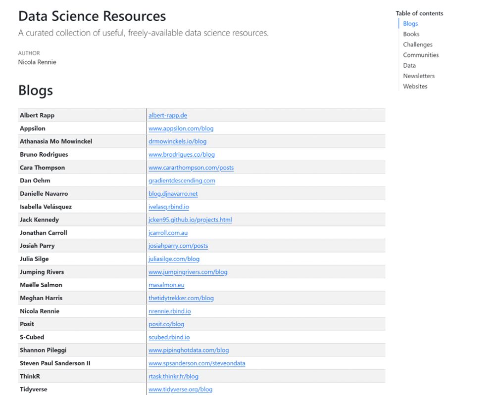
October 18, 2024 at 1:58 PM
I've recently started compiling a list of data science related resources that I use or recommend frequently! 📊
Link: nrennie.rbind.io/data-science...
#RStats #Python #DataViz #DataScience
Link: nrennie.rbind.io/data-science...
#RStats #Python #DataViz #DataScience
My position in public administration could easily be labeled 'Macrodata Refinement' at Lumon like in Severance. Just waiting for the chip to be installed so I can finally achieve optimal work-life separation

a woman with red hair is wearing a blue top
ALT: a woman with red hair is wearing a blue top
media.tenor.com
June 21, 2025 at 9:49 AM
My position in public administration could easily be labeled 'Macrodata Refinement' at Lumon like in Severance. Just waiting for the chip to be installed so I can finally achieve optimal work-life separation

Un bon exemple de com un usuari de Python veu les virtuts d'R
borkar.substack.com/p/unlocking-....
Ara només falta que un usuari com jo d'R li vegi les virtuts a Python, que estic seguríssim que en té
borkar.substack.com/p/unlocking-....
Ara només falta que un usuari com jo d'R li vegi les virtuts a Python, que estic seguríssim que en té

Unlocking Zen: How R's data analysis ecosystem outshines Python
In this article, I highlight some pain-points when working with Python & Pandas and how R's ecosystem proves to be a great alternative.
borkar.substack.com
June 1, 2025 at 9:00 AM
Un bon exemple de com un usuari de Python veu les virtuts d'R
borkar.substack.com/p/unlocking-....
Ara només falta que un usuari com jo d'R li vegi les virtuts a Python, que estic seguríssim que en té
borkar.substack.com/p/unlocking-....
Ara només falta que un usuari com jo d'R li vegi les virtuts a Python, que estic seguríssim que en té
A gerardreverte.github.io/estoc_person... ja podeu trobar el codi de l'script d'R per calcular l'estoc de persones. No és totalment reproduïble ja que les dades estan guardades en una base de dades "duckdb" en local, però menys és res.😅
@ekotov.pro @josepvives.bsky.social @toni-salvado.bsky.social
@ekotov.pro @josepvives.bsky.social @toni-salvado.bsky.social
Estoc de persones als municipis de l’Estat espanyol
gerardreverte.github.io
May 29, 2025 at 11:36 AM
A gerardreverte.github.io/estoc_person... ja podeu trobar el codi de l'script d'R per calcular l'estoc de persones. No és totalment reproduïble ja que les dades estan guardades en una base de dades "duckdb" en local, però menys és res.😅
@ekotov.pro @josepvives.bsky.social @toni-salvado.bsky.social
@ekotov.pro @josepvives.bsky.social @toni-salvado.bsky.social
🧵 1/9 📊 Dades obertes del MITMS ens permeten saber quanta gent hi havia a cada municipi en cada moment. Mobilitat, esdeveniments, hàbits socials! 💡Periodistes i urbanistes:
@elivivas.bsky.social @drxeo.eu @rogertugas.bsky.social
@kikollan.llaneras.es
📍Exemples 👇
@elivivas.bsky.social @drxeo.eu @rogertugas.bsky.social
@kikollan.llaneras.es
📍Exemples 👇
May 26, 2025 at 4:19 PM
🧵 1/9 📊 Dades obertes del MITMS ens permeten saber quanta gent hi havia a cada municipi en cada moment. Mobilitat, esdeveniments, hàbits socials! 💡Periodistes i urbanistes:
@elivivas.bsky.social @drxeo.eu @rogertugas.bsky.social
@kikollan.llaneras.es
📍Exemples 👇
@elivivas.bsky.social @drxeo.eu @rogertugas.bsky.social
@kikollan.llaneras.es
📍Exemples 👇
De veritat que això no és un genocidi?
www.bbc.com/news/live/c1...
www.bbc.com/news/live/c1...

'Children cry from hunger - their mothers have nothing to feed them': Gazans speak to BBC
Israel says it's blocking aid to put pressure on Hamas to release hostages, but aid agencies accuse it of using starvation as a weapon of war.
www.bbc.com
May 15, 2025 at 4:01 PM
De veritat que això no és un genocidi?
www.bbc.com/news/live/c1...
www.bbc.com/news/live/c1...
Reposted by Gerard Reverté

#dataviz
"BEL, the difference between the highest and lowest rate is almost 30 percentage points, the most progressive in
Most western countries likewise have a fairly progressive range (>20pp)
SPA has lowest for the poorest households (6.5%), (21.9pp range)"
www.datawrapper.de/blog/progres...
"BEL, the difference between the highest and lowest rate is almost 30 percentage points, the most progressive in
Most western countries likewise have a fairly progressive range (>20pp)
SPA has lowest for the poorest households (6.5%), (21.9pp range)"
www.datawrapper.de/blog/progres...

Flat out unfair? A progressive take on taxes | Datawrapper Blog
Hi, this is Luc, working in the visualization team. If you like visualizing data …
www.datawrapper.de
May 8, 2025 at 5:34 PM
#dataviz
"BEL, the difference between the highest and lowest rate is almost 30 percentage points, the most progressive in
Most western countries likewise have a fairly progressive range (>20pp)
SPA has lowest for the poorest households (6.5%), (21.9pp range)"
www.datawrapper.de/blog/progres...
"BEL, the difference between the highest and lowest rate is almost 30 percentage points, the most progressive in
Most western countries likewise have a fairly progressive range (>20pp)
SPA has lowest for the poorest households (6.5%), (21.9pp range)"
www.datawrapper.de/blog/progres...
Imprescindible llegir aquest article de Siri Hustvedt a El Pais
bsky.app/profile/elpa...
bsky.app/profile/elpa...

Tribuna | "Las palabras importan. Las palabras son acción. Hablar y escribir públicamente, o en la clandestinidad si se agrava la represión, será crucial para contribuir a que la segunda versión de Trump conserve o pierda su autoridad", por la escritora Siri Hustvedt

El fascismo en Estados Unidos | Tribuna
Las palabras importan, alteran la percepción, excitan las emociones y serán cruciales para influir en el rumbo de los acontecimientos políticos
elpais.com
April 18, 2025 at 7:41 AM
Imprescindible llegir aquest article de Siri Hustvedt a El Pais
bsky.app/profile/elpa...
bsky.app/profile/elpa...
Absolutament increïble!!!😖😖
bsky.app/profile/miqu...
bsky.app/profile/miqu...

I received a heartbreaking email today: A paper in a special issue I’m editing is being retracted because one of its authors is afraid of losing their job and their legal status in the U.S. if they publish a scientific study on evolution. Yes, on evolution, nature's engine of diversity.
March 30, 2025 at 10:25 AM
Absolutament increïble!!!😖😖
bsky.app/profile/miqu...
bsky.app/profile/miqu...
Reposted by Gerard Reverté

library(legendry)
histogram_guide <- compose_sandwich(
middle = gizmo_histogram(just = 0),
text = "axis_base",
position = "bottom"
)
nc <- sf::st_read(system.file("shape/nc.shp", package = "sf"), quiet = TRUE)
ggplot(nc) +
geom_sf(aes(fill = AREA)) +
guides(fill = histogram_guide)
histogram_guide <- compose_sandwich(
middle = gizmo_histogram(just = 0),
text = "axis_base",
position = "bottom"
)
nc <- sf::st_read(system.file("shape/nc.shp", package = "sf"), quiet = TRUE)
ggplot(nc) +
geom_sf(aes(fill = AREA)) +
guides(fill = histogram_guide)

February 18, 2025 at 5:44 PM
library(legendry)
histogram_guide <- compose_sandwich(
middle = gizmo_histogram(just = 0),
text = "axis_base",
position = "bottom"
)
nc <- sf::st_read(system.file("shape/nc.shp", package = "sf"), quiet = TRUE)
ggplot(nc) +
geom_sf(aes(fill = AREA)) +
guides(fill = histogram_guide)
histogram_guide <- compose_sandwich(
middle = gizmo_histogram(just = 0),
text = "axis_base",
position = "bottom"
)
nc <- sf::st_read(system.file("shape/nc.shp", package = "sf"), quiet = TRUE)
ggplot(nc) +
geom_sf(aes(fill = AREA)) +
guides(fill = histogram_guide)
Reposted by Gerard Reverté

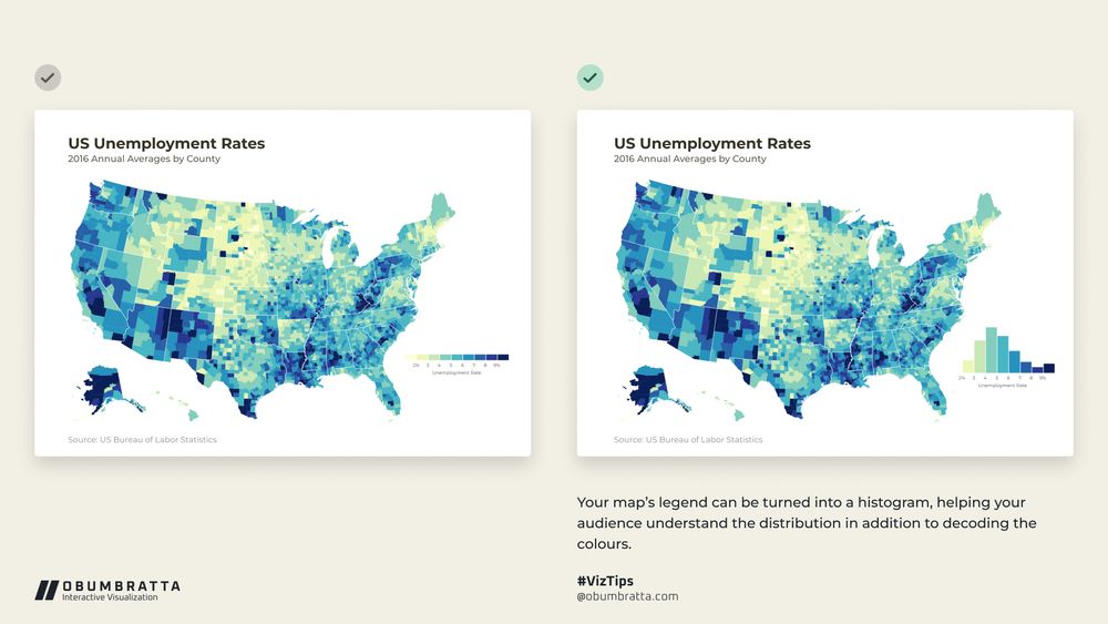
Your map’s legend can be turned into a histogram, helping your audience understand the distribution in addition to decoding the colours.
November 25, 2024 at 6:38 PM
Your map’s legend can be turned into a histogram, helping your audience understand the distribution in addition to decoding the colours.
Reposted by Gerard Reverté

El Local Neighbourhood Gini (LNG) és una nova mesura de la desigualtat local independent dels límits administratius que utilitza dades geolocalitzades d'habitatge
https://www.sciencedirect.com/science/article/pii/S004727272400224X
https://www.sciencedirect.com/science/article/pii/S004727272400224X

February 5, 2025 at 5:31 AM
El Local Neighbourhood Gini (LNG) és una nova mesura de la desigualtat local independent dels límits administratius que utilitza dades geolocalitzades d'habitatge
https://www.sciencedirect.com/science/article/pii/S004727272400224X
https://www.sciencedirect.com/science/article/pii/S004727272400224X
Reposted by Gerard Reverté

This is a big deal, y'all. Federal health websites are being stripped of content or removed in their entirety. Stick with this thread for a look at what's disappeared so far! 1/x
January 31, 2025 at 7:28 PM
This is a big deal, y'all. Federal health websites are being stripped of content or removed in their entirety. Stick with this thread for a look at what's disappeared so far! 1/x
Reposted by Gerard Reverté