


Robert Rosenbaum
@robertrosenbaum.bsky.social
Associate Professor of Applied and Computational Mathematics and Statistics and Biological Sciences at U Notre Dame. Theoretically a Neuroscientist.
Finally, we meta-learned pure plasticity rules with no weight transport, extending our previous work. When Oja's rule was included, the meta-learned rule _outperformed_ pure backprop.

May 19, 2025 at 3:33 PM
Finally, we meta-learned pure plasticity rules with no weight transport, extending our previous work. When Oja's rule was included, the meta-learned rule _outperformed_ pure backprop.
We find that Oja's rule works, in part, by preserving information about inputs in hidden layers. This is related to its known properties in forming orthogonal representations. Check the paper for more details.

May 19, 2025 at 3:33 PM
We find that Oja's rule works, in part, by preserving information about inputs in hidden layers. This is related to its known properties in forming orthogonal representations. Check the paper for more details.
Vanilla RNNs trained with pure BPTT fail on simple memory tasks. Adding Oja's rule to BPTT drastically improves performance.

May 19, 2025 at 3:33 PM
Vanilla RNNs trained with pure BPTT fail on simple memory tasks. Adding Oja's rule to BPTT drastically improves performance.
We often forget how important careful weight initialization is for training neural nets because our software initializes them for us. Adding Oja's rule to backprop also eliminates the need for careful weight initialization.

May 19, 2025 at 3:33 PM
We often forget how important careful weight initialization is for training neural nets because our software initializes them for us. Adding Oja's rule to backprop also eliminates the need for careful weight initialization.
We propose that plasticity rules like Oja's rule might be part of the answer. Adding Oja's rule to backprop improves learning in deep networks in an online setting (batch size 1).

May 19, 2025 at 3:33 PM
We propose that plasticity rules like Oja's rule might be part of the answer. Adding Oja's rule to backprop improves learning in deep networks in an online setting (batch size 1).
For example, a 10-layer ffwd network trained on MNIST using online learning (batch size 1) performs poorly when trained with pure backprop. How does the brain learn effectively without all of these engineering hacks?

May 19, 2025 at 3:33 PM
For example, a 10-layer ffwd network trained on MNIST using online learning (batch size 1) performs poorly when trained with pure backprop. How does the brain learn effectively without all of these engineering hacks?
In previous work on this question, we meta-learned linear combos of plasticity rules. In doing so, we noticed something intersting:
One plasticity rule improved learning, but its weight updates weren't aligned with backprop's. It was doing something different. That rule is Oja's plasticity rule.
One plasticity rule improved learning, but its weight updates weren't aligned with backprop's. It was doing something different. That rule is Oja's plasticity rule.

May 19, 2025 at 3:33 PM
In previous work on this question, we meta-learned linear combos of plasticity rules. In doing so, we noticed something intersting:
One plasticity rule improved learning, but its weight updates weren't aligned with backprop's. It was doing something different. That rule is Oja's plasticity rule.
One plasticity rule improved learning, but its weight updates weren't aligned with backprop's. It was doing something different. That rule is Oja's plasticity rule.
A lot of work in "NeuroAI," including our own, seeks to understand how synaptic plasticity rules can match the performance of backprop in training neural nets.

May 19, 2025 at 3:33 PM
A lot of work in "NeuroAI," including our own, seeks to understand how synaptic plasticity rules can match the performance of backprop in training neural nets.
Thanks. Yeah, I think this example helps clarify 2 points:
1) large negative eigenvalues are not necessary for LRS, and
2) high-dim input and stable dynamics are not sufficient for high-dim responses.
Motivated by this conversation, I added eigenvalues to the plot and edited the text a bit, thx!
1) large negative eigenvalues are not necessary for LRS, and
2) high-dim input and stable dynamics are not sufficient for high-dim responses.
Motivated by this conversation, I added eigenvalues to the plot and edited the text a bit, thx!
May 2, 2025 at 4:51 PM
Thanks. Yeah, I think this example helps clarify 2 points:
1) large negative eigenvalues are not necessary for LRS, and
2) high-dim input and stable dynamics are not sufficient for high-dim responses.
Motivated by this conversation, I added eigenvalues to the plot and edited the text a bit, thx!
1) large negative eigenvalues are not necessary for LRS, and
2) high-dim input and stable dynamics are not sufficient for high-dim responses.
Motivated by this conversation, I added eigenvalues to the plot and edited the text a bit, thx!
High-dim dynamics has additional constraints. but when the low rank part has rank>1, it's not just negative overlaps between sing vecs. Instead, the "overlap matrix" needs to lack small singular values.
Attached is an example (Fig 2d,e in paper) with pos and neg overlaps (P is the overlap matrix).
Attached is an example (Fig 2d,e in paper) with pos and neg overlaps (P is the overlap matrix).

April 26, 2025 at 12:39 PM
High-dim dynamics has additional constraints. but when the low rank part has rank>1, it's not just negative overlaps between sing vecs. Instead, the "overlap matrix" needs to lack small singular values.
Attached is an example (Fig 2d,e in paper) with pos and neg overlaps (P is the overlap matrix).
Attached is an example (Fig 2d,e in paper) with pos and neg overlaps (P is the overlap matrix).
I don't think your reduction to eigenvalues does not capture everything, though.
For example, LRS is very general, occurs in the attached example where the dominant left- and right singular vectors are near-orthogonal. E-vals are negative, but O(1) in magnitude, not separated from bulk.
For example, LRS is very general, occurs in the attached example where the dominant left- and right singular vectors are near-orthogonal. E-vals are negative, but O(1) in magnitude, not separated from bulk.

April 26, 2025 at 12:39 PM
I don't think your reduction to eigenvalues does not capture everything, though.
For example, LRS is very general, occurs in the attached example where the dominant left- and right singular vectors are near-orthogonal. E-vals are negative, but O(1) in magnitude, not separated from bulk.
For example, LRS is very general, occurs in the attached example where the dominant left- and right singular vectors are near-orthogonal. E-vals are negative, but O(1) in magnitude, not separated from bulk.
To clarify before I continue:
LRS is defined as the presence of a small number of suppressed directions (the last blue dot in the var expl figure we are replying to).
High-dim responses is the absence of a small number of amplified directions.
I attached our assumptions and conditions for each.
LRS is defined as the presence of a small number of suppressed directions (the last blue dot in the var expl figure we are replying to).
High-dim responses is the absence of a small number of amplified directions.
I attached our assumptions and conditions for each.

April 26, 2025 at 12:39 PM
To clarify before I continue:
LRS is defined as the presence of a small number of suppressed directions (the last blue dot in the var expl figure we are replying to).
High-dim responses is the absence of a small number of amplified directions.
I attached our assumptions and conditions for each.
LRS is defined as the presence of a small number of suppressed directions (the last blue dot in the var expl figure we are replying to).
High-dim responses is the absence of a small number of amplified directions.
I attached our assumptions and conditions for each.
Real epidemiological dynamics are subject to noise (eg, interactions with individuals outside the network).
If we account for this, the network produces high-dim dynamics.
And the network is more sensitive to random perturbations than to perturbations aligned to the low dim structure.
If we account for this, the network produces high-dim dynamics.
And the network is more sensitive to random perturbations than to perturbations aligned to the low dim structure.

April 21, 2025 at 5:00 PM
Real epidemiological dynamics are subject to noise (eg, interactions with individuals outside the network).
If we account for this, the network produces high-dim dynamics.
And the network is more sensitive to random perturbations than to perturbations aligned to the low dim structure.
If we account for this, the network produces high-dim dynamics.
And the network is more sensitive to random perturbations than to perturbations aligned to the low dim structure.
Network's with spatial structure also have low rank parts that are EP.
Due to low-rank suppression these networks amplify spatially disordered inputs relative to spatially smooth ones.
Due to low-rank suppression these networks amplify spatially disordered inputs relative to spatially smooth ones.

April 21, 2025 at 5:00 PM
Network's with spatial structure also have low rank parts that are EP.
Due to low-rank suppression these networks amplify spatially disordered inputs relative to spatially smooth ones.
Due to low-rank suppression these networks amplify spatially disordered inputs relative to spatially smooth ones.
Networks with modular structure have low-rank parts that are not necessarily normal, but it is EP.
Due to low-rank suppression, these networks amplify random input relative to inputs that are homogeneous within each module.
This effect is related to E-I balance in neural circuits.
Due to low-rank suppression, these networks amplify random input relative to inputs that are homogeneous within each module.
This effect is related to E-I balance in neural circuits.

April 21, 2025 at 5:00 PM
Networks with modular structure have low-rank parts that are not necessarily normal, but it is EP.
Due to low-rank suppression, these networks amplify random input relative to inputs that are homogeneous within each module.
This effect is related to E-I balance in neural circuits.
Due to low-rank suppression, these networks amplify random input relative to inputs that are homogeneous within each module.
This effect is related to E-I balance in neural circuits.
This can be understood intuitively by looking at the steady state (or quasi-steady state) network state.
The steady state is determined by the input through multiplication by the inverse of the network's connectivity matrix.
The steady state is determined by the input through multiplication by the inverse of the network's connectivity matrix.

April 21, 2025 at 5:00 PM
This can be understood intuitively by looking at the steady state (or quasi-steady state) network state.
The steady state is determined by the input through multiplication by the inverse of the network's connectivity matrix.
The steady state is determined by the input through multiplication by the inverse of the network's connectivity matrix.
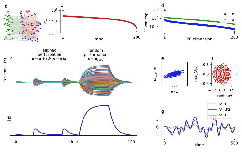
To illustrate low-rank suppression, consider the same network subject to two different perturbations:
One is aligned to the low dimensional structure of the network.
The other is random.
Perhaps surprisingly, the network's response to the aligned stimulus is suppressed relative to the random one.
One is aligned to the low dimensional structure of the network.
The other is random.
Perhaps surprisingly, the network's response to the aligned stimulus is suppressed relative to the random one.

April 21, 2025 at 5:00 PM
To illustrate low-rank suppression, consider the same network subject to two different perturbations:
One is aligned to the low dimensional structure of the network.
The other is random.
Perhaps surprisingly, the network's response to the aligned stimulus is suppressed relative to the random one.
One is aligned to the low dimensional structure of the network.
The other is random.
Perhaps surprisingly, the network's response to the aligned stimulus is suppressed relative to the random one.
If you're not surprised by the low-dim network's high-dim response to a high-dim input, there is another surprise in store.
Notice the last PC of the dynamics (last blue dot):
There is an abrupt jump downward in var explained.
This is caused by an effect we call "low-rank suppression"
Notice the last PC of the dynamics (last blue dot):
There is an abrupt jump downward in var explained.
This is caused by an effect we call "low-rank suppression"

April 21, 2025 at 5:00 PM
If you're not surprised by the low-dim network's high-dim response to a high-dim input, there is another surprise in store.
Notice the last PC of the dynamics (last blue dot):
There is an abrupt jump downward in var explained.
This is caused by an effect we call "low-rank suppression"
Notice the last PC of the dynamics (last blue dot):
There is an abrupt jump downward in var explained.
This is caused by an effect we call "low-rank suppression"
Perhaps counter to intuition, dynamics on the network were high-dimensional:
The variance explained by the principal components of the network dynamics (blue) decayed slowly, reflecting those of of the stimulus (green), but not the network structure (red above).
The variance explained by the principal components of the network dynamics (blue) decayed slowly, reflecting those of of the stimulus (green), but not the network structure (red above).

April 21, 2025 at 5:00 PM
Perhaps counter to intuition, dynamics on the network were high-dimensional:
The variance explained by the principal components of the network dynamics (blue) decayed slowly, reflecting those of of the stimulus (green), but not the network structure (red above).
The variance explained by the principal components of the network dynamics (blue) decayed slowly, reflecting those of of the stimulus (green), but not the network structure (red above).
We started with a simple example: A recurrent network with one-dimensional structure and linear dynamics.
We perturbed the network with a high-dimensional input (iid smooth Gaussian noise).
We perturbed the network with a high-dimensional input (iid smooth Gaussian noise).

April 21, 2025 at 5:00 PM
We started with a simple example: A recurrent network with one-dimensional structure and linear dynamics.
We perturbed the network with a high-dimensional input (iid smooth Gaussian noise).
We perturbed the network with a high-dimensional input (iid smooth Gaussian noise).
Work by @computingnature.bsky.social, @marius10p.bsky.social, and others showed that neural populations in the brain produce high-dimensional dynamics when in response to high-dimensional stimuli.
High-dimensional stimuli produce high-dimensional dynamics.
High-dimensional stimuli produce high-dimensional dynamics.

April 21, 2025 at 5:00 PM
Work by @computingnature.bsky.social, @marius10p.bsky.social, and others showed that neural populations in the brain produce high-dimensional dynamics when in response to high-dimensional stimuli.
High-dimensional stimuli produce high-dimensional dynamics.
High-dimensional stimuli produce high-dimensional dynamics.
Recent work by Vincent Thibeault, @allard.bsky.social, and Patrick Desrosiers shows that many networks arising in nature have an (approximate) low dimensional structure in the sense that the singular values of their adjacency matrices are dominated by a small number of large values.

April 21, 2025 at 5:00 PM
Recent work by Vincent Thibeault, @allard.bsky.social, and Patrick Desrosiers shows that many networks arising in nature have an (approximate) low dimensional structure in the sense that the singular values of their adjacency matrices are dominated by a small number of large values.
High-Dimensional Dynamics in Low-Dimensional Networks.
New preprint with a former undergrad, Yue Wan.
I'm not totally sure how to talk about these results. They're counterintuitive on the surface, seem somewhat obvious in hindsight, but then there's more to them when you dig deeper.
New preprint with a former undergrad, Yue Wan.
I'm not totally sure how to talk about these results. They're counterintuitive on the surface, seem somewhat obvious in hindsight, but then there's more to them when you dig deeper.

April 21, 2025 at 5:00 PM
High-Dimensional Dynamics in Low-Dimensional Networks.
New preprint with a former undergrad, Yue Wan.
I'm not totally sure how to talk about these results. They're counterintuitive on the surface, seem somewhat obvious in hindsight, but then there's more to them when you dig deeper.
New preprint with a former undergrad, Yue Wan.
I'm not totally sure how to talk about these results. They're counterintuitive on the surface, seem somewhat obvious in hindsight, but then there's more to them when you dig deeper.
Additional topics and models are covered in a second appendix.

January 27, 2025 at 6:20 PM
Additional topics and models are covered in a second appendix.
The main text covers a minimal thread of concepts needed to build up from ion channels to neural networks.
The book assumes no background in biology, only a basic background in math (e.g., calculus and matrices).
All other mathematical background is covered in an appendix.
(3/n)
The book assumes no background in biology, only a basic background in math (e.g., calculus and matrices).
All other mathematical background is covered in an appendix.
(3/n)

January 27, 2025 at 6:20 PM
The main text covers a minimal thread of concepts needed to build up from ion channels to neural networks.
The book assumes no background in biology, only a basic background in math (e.g., calculus and matrices).
All other mathematical background is covered in an appendix.
(3/n)
The book assumes no background in biology, only a basic background in math (e.g., calculus and matrices).
All other mathematical background is covered in an appendix.
(3/n)